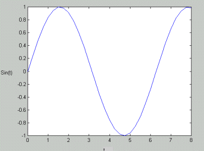
Figure (1) - Sin (t) function
Arrays and their operations
Matrix and their operations
Some Linear Algebra in Matlab
In this lab you will learn about some of the commands
used in Matlab.
You can cut and paste most of the instructions in this lab manual to the Matlab prompt or to the .m file.
Values for t:
0 0.2500 0.5000
0.7500 1.0000 1.2500
1.5000 1.7500 2.0000 2.2500
2.5000 2.7500 3.0000
3.2500 3.5000 3.7500 4.0000
4.2500 4.5000 4.7500
5.0000 5.2500 5.5000 5.7500
6.0000 6.2500 6.5000
6.7500 7.0000 7.2500 7.5000
7.7500 8.0000
Corresponding sin(t) values:
0 0.2474 0.4794
0.6816 0.8415 0.9490
0.9975 0.9840 0.9093 0.7781
0.5985 0.3817 0.1411 -0.1082
-0.3508 -0.5716 -0.7568 -0.8950
-0.9775 -0.9993 -0.9589 -0.8589
-0.7055 -0.5083 -0.2794 -0.0332
0.2151 0.4500 0.6570 0.8231
0.9380 0.9946 0.9894

Figure (1) - Sin (t) function
As you can see t is a set of numbers (1-D array) so as sin(t) corresponding to the t values. In Matlab this operation can be done very easy. Here is how we could create vector t, at the Matlab prompt, type:
Creating an array:
t = [0 0.25 0.5 0.75 1.0 1.25 1.5 1.75 2.0 2.25 2.50 2.75
3.00 3.25 3.5 3.75 4.0 4.25 4.5 4.75 5.0 5.25
5.5 5.75 6.0 6.25 6.5 6.75 7.0 7.25
7.50 7.750 8.0]
This will generate an output that looks like this:
t =
Columns 1 through 7
0
0.2500 0.5000 0.7500
1.0000 1.2500 1.5000
Columns 8 through 14
1.7500 2.0000
2.2500 2.5000 2.7500
3.0000 3.2500
Columns 15 through 21
3.5000 3.7500
4.0000 4.2500 4.5000
4.7500 5.0000
Columns 22 through 28
5.2500 5.5000
5.7500 6.0000 6.2500
6.5000 6.7500
Columns 29 through 33
7.0000 7.2500
7.5000 7.7500 8.0000
There are many built-in functions in Matlab, for example: sin, cos, sqrt, .... Matlab even allows you to add your own function. Let's use the above numbers to generate the sin(t). In order to do this, at the prompt, type y = sin(t). Note how this will work, since t is an array, then y will be an array that holds exactly the same number of elements, y = sin(t), corresponding to each one of t values. The result will be:
Using a function:
» y = sin(t)
y =
Columns 1 through 7
0
0.2474 0.4794 0.6816
0.8415 0.9490 0.9975
Columns 8 through 14
0.9840 0.9093
0.7781 0.5985 0.3817
0.1411 -0.1082
Columns 15 through 21
-0.3508 -0.5716 -0.7568
-0.8950 -0.9775 -0.9993 -0.9589
Columns 22 through 28
-0.8589 -0.7055 -0.5083
-0.2794 -0.0332 0.2151
0.4500
Columns 29 through 33
0.6570 0.8231
0.9380 0.9946 0.9894
Please note that to clear values of t from the memory, you need to type >> clear t.
As you perhaps noticed in the above example, t started from 0 and went up 0.25 by 0.25 until we got to 8. We can use a different method to generate t values and avoid typing all those numbers.
Another method for creating the same array:
>> t = 0:0.25:8
This will result in the same numbers for t as you had before.
Then, you can generate the sin(t) values in the same way as before.
>> y = sin(t).
A quick note: All angles must be represented in Radian.
In order to do this, you have to use (x*pi/180). For instance, sin(45)
= 0.7071, but if you type:
>> sin(45) you will get 0.8509. In order to get the right answer
you have to type:
>> y = sin(45*pi/180), which results into the right answer, 0.7071.
Manipulation of arrays:
Suppose, we want to compute sin(2t). Notice that you want to
do this for all sin values. If you wanted to do this in C++, you
would use a loop to go through all t values and you would multiply the
values by 2, then you would compute sin(2t) . But here, this done
much easier and faster.
>> clear t
>> clear y
>> t = 0:0.25:8
>> z = t + t
>> y = sin(z)
Problem (1) : sin(2t) = 2 sin(t)cos(t). Use Matlab to find the values for sin(2t) using the above procedure and using 2sin(t)cos(t). Confirm that both methods generate the same results.
Problem (1) G. (Graduate students only) : sin2(t) + cos2(t) = 1, use matlab to do this using array operations.
Suppose we have a 3x3 matrix, A, defined as;
A =
20 22 18
12 16 12
8 10 10
and another one with the same size, B, defined as;
B =
2 4 8
1 -1 6
-2 2 4
How do we enter these matrices in Matlab.
First method:
A = [20 22 18; 12 16 12; 8 10 10]
The output will looks like this:
A =
20 22 18
12 16 12
8 10 10
Second method:
B =
[2 4 8
1 -1 6
-2 2 4]
The output looks like this:
B =
2 4
8
1 -1
6
2 2
4
Let's try few of the operations in linear algebra here.
Suppose, you want to find the transpose of matrix A, rows are interchanged
with columns, and call the new matrix C.
>> C = A'
This generates the following output;
C =
20 12
8
22 16 10
18 12 10
Problem (2) If A was a complex matrix, what procedure would you use to generate its transpose? and what was the outcome of the transpose operation in that case?.
Suppose, we want to compute D = A * B. Do
you remember how that is done ?
>> D = A*B
D =
98 94 364
64 56 240
46 42 164
Problem (3) How do you multiply the corresponding elements of matrix A and B ? Please note that I didn't ask you to multiply A * B. I want you to tell me how to multiply A(1,1) by B(1,1), and A(1,2) by B(1,2), ....? Find the results of your work.
Problem (3) G. How do you find the cube of matrix A? One way is to multiply A by itself 3 times, but there is an easier way using Matlab commands.
You can also find the inverse of a matrix:
>> X = inv(A)
X =
0.3125 -0.3125 -0.1875
-0.1875 0.4375 -0.1875
-0.0625 -0.1875 0.4375
Did you know how much work you needed to do if you wanted to do this using traditional method? How do we compute the inverse matrix anyway?
We can find the eigenvalues of a matrix too.
>> eig(A)
ans =
42.4939
2.0000
1.5061
There is even a function to find the coefficients of the characteristic polynomial of a matrix. The "poly" function creates a vector that includes the coefficients of the characteristic polynomial.
>> p = poly(A)
Answer is:
p =
1.0000 -46.0000 152.0000 -128.0000
We can find the roots of the characteristic polynomial, which is the
same as eigenvalues:
>> roots(p)
ans =
42.4939
2.0000
1.5061
ns = 5.3723 -0.3723
In this lab, you tried several of the Matlab commands individually. You could put all of the commands that you want to execute together in a m-file, and just run the file. If you put all of your m-files in the same directory that you run matlab from, then Matlab will always find them.