 takes (x,y) to (1/2 x + 1/2 y, 1/2 x +1/2 y), ie projected onto the y=x
line. If we look at light rays perpendicular to the y=x line, this matrix
gives
us the shadow a vector makes onto the y=x line, which has
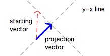
many applications in mathematics and physics. In other words, given
a starting vector,
we drop the perpendicular to the y=x line, and the base of the
right triangle we form is the projection vector.
takes (x,y) to (1/2 x + 1/2 y, 1/2 x +1/2 y), ie projected onto the y=x
line. If we look at light rays perpendicular to the y=x line, this matrix
gives
us the shadow a vector makes onto the y=x line, which has
many applications in mathematics and physics. In other words, given
a starting vector,
we drop the perpendicular to the y=x line, and the base of the
right triangle we form is the projection vector.
Execute with(LinearAlgebra): Enter M into Maple. Use commands like
M.Vector([-1, 1]);
to test M on different column vectors like (1,0), (0,1), (1,1), and (-1,1). Notice that any vectors on the lines y=x and y=-x, with basis representatives (1,1) and (-1,1), are eigenvectors for M. In addition, (-1,1) or anything else on the line y=-x gets sent to (0,0) which is still on the same line through the origin, so the eigenvalue is 0, and anything on y=x, like (1,1) gets fixed by M, so the eigenvalue is 1.]
A:=Matrix([[(cos(theta))^2,cos(theta)*sin(theta)],[cos(theta)*sin(theta),((sin(theta))^2)]]);
The matrix A projects vectors onto the line through the origin that makes an angle of theta degrees with the positive x-axis [in number 1 above, the line was y=x, ie theta was 45 degrees from the positive x-axis. In this case sin and cos are sqrt(2)/2, so the matrix has all entries of 1/2 like M does].
Let's use a bit of trigonometry to determine the equation of the line of projection for A for a general theta:
Notice that theta is labeled in the picture above, and I have created a right triangle to the x-axis so that we can use the trigonometry of the unit circle. The hypotenuse is the line of projection for A. Why is the x-value of point P in the picture above cos(theta)? Why is the y-value sin(theta)? Use this to show that the slope of the hypotenuse from (0,0) to P=(cos(theta), sin(theta)) is tan(theta). Since the y-intercept occurs at (0,0), this would tell us that the line of projection is y=tan(theta) x.
We use some pictures to help interpret the result:
theta=Pi/4 First, when theta is Pi/4, as in #1 above, here is the input (red) and output (blue) picture for one vector. Notice that the red vector is projected onto the y=tan(theta) x line via its shadow.
 We place the output vectors
in blue at the tail of the unit circle
input vectors for ease of visualizing them all at
once:
We place the output vectors
in blue at the tail of the unit circle
input vectors for ease of visualizing them all at
once:
theta=Pi/4
We can identify the eigenvectors by looking for vectors which stay on the same line through the origin, and we can identify the eigenvalues by how they are scaled along that line. You should be able to see that the only vectors that stay on the same line through the origin are (1,1) which gets fixed since it is on the line of projection (eigenvalue 1) and (-1,1) which has no shadow since it is perpendicular to the line of projection (eigenvalue 0). Everything else in that picture ends up on a different line it started on.
theta=Pi/2 When theta is Pi/2, the line of projection is the y-axis
theta=Pi/2
What are the eigenvectors and eigenvalues in this case? You should be able to identify them from the picture.
Execute
theta := Pi/2
in Maple, and then execute
Eigenvectors(A);
and compare with the above picture. The eigenvalue of 1 corresponds to vectors on the line of projection, and the eigenvalue of 0 corresponds to vectors perpendicular to the line of projection.
theta=Pi/1.8 and here is the picture for theta equal to Pi/1.8:
theta=Pi/1.8
Where in the picture is the eigenvector corresponding to 1? How does this relate to the line of projection y=tan(Pi/1.8) x?
Where in the picture is the eigenvector corresponding to 0? How does this relate to the line of projection?
Note that if you wish to try theta := Pi/(1.8); Eigenvectors(A); in Maple, this won't help us much since Maple will tell use it wants rational values. An evalf of the angle is a bit more fruitful, but we pick up some rounding issues, like -.984807753000000008+0.I
However we can use a geometric explanation to explain what the eigenvectors are for theta=Pi/1.8: Vectors on the line of projection are fixed so they have eigenvalue 1. In this case an eigenvector is P = (cos(theta),sin(theta)) = (cos(Pi/1.8), sin(Pi/1.8))
.
Vectors perpendicular to the line of projection have no shadow so they have
eigenvalue 0. How do we find a vector perpendicular to
 ? Hint - we need the slope to be the negative
reciprocal.
? Hint - we need the slope to be the negative
reciprocal.
 and input P into Maple via
theta := 'theta'
P:=Matrix...
Note that the first command resets theta.
Use only a geometric explanation, similar to the explanation for Pi/1.8 above, to explain why the first column is an eigenvector corresponding to the eigenvalue of 1, and why the second column is an eigenvector corresponding to an eigenvector of 0.
What familiar geometric transformation is P? How about MatrixInverse(P)?
Diag:=simplify(MatrixInverse(P).A.P)
What familiar geometric transformation is Diag?
If we want to project a vector onto the y=tan(theta) x line, first we can perform MatrixInverse(P) which takes a vector and rotates it ___________________ by theta. Next we perform Diag, which projects onto the line _____________ . And finally we perform P, which rotates ___________________ by theta.
It is sometimes easier to visualize by using a point on the y=tan(theta) x line, which we know is fixed under the projection. So take the vector (cos(theta),sin(theta)). Use matrix multiplication in Maple or geometric intuition to fill in these blanks: MatrixInverse(P) takes this point to the point ________________. Next we perform Diag which gives us the point _______________. Finally, we perform P, which takes the point back where we started to (cos(theta),sin(theta)).
Part A: Execute the Eigenvectors command.
Part B: Let the matrix act on a column vector (x,y) via matrix multiplication.
Part C: How does this transformation act on R2?
Part D: Use Part C to explain your output in Part A.
Sh:=Matrix([[1,k],[0,1]]);
Part A: Execute the Eigenvectors command.
Part B: Let the matrix act on a column vector (x,y) via matrix multiplication.
Part C: Test out the image of a square with vertices (1,0), (1,1), (2,0), (2,1). What does Sh do to this square for k = 1? For k=2?
Part D: How does Sh act as a transformation on R2 for positive k values?
Part E: Use Part D to explain your output in Part A.
Part F: Is A diagonalizable? Why or why not?
Part G: If k=0, Maple's response to Part A and your response to Part F are both incorrect - what should the responses be?
Sv:=Matrix([[1,0],[k,1]]);
Repeat Parts A, B, D, and E for this matrix.
R:=Matrix([[cos(theta), sin(theta)],[sin(theta), -cos(theta)]]);
Notice the difference between this matrix and P in #5 above.
Part A: Apply the Eigenvectors(R); and Eigenvalues(R); commands. Notice that Maple will not output the eigenvectors, but it will output the eigenvalues.
Part B: When theta=0, what geometric transformation is R? What are the eigenvectors for each eigenvalue in this case?
Part C: When theta=Pi/2, what geometric transformation is R? What are the eigenvectors for each eigenvalue in this case?
Part D: When theta=Pi, what geometric transformation is R? What are the eigenvectors for each eigenvalue in this case?
Part E: What is the relationship between theta and the geometric transformation R(theta)?
Part F: What are the eigenvectors for each eigenvalue for a general theta (hint: the reasoning and trigonometry is similar to what we used in the projection matrix questions 2 and 5)
Part G: Is R(theta) diagonalizable?