In part 1 of chapter 7 group work we found that the eigenvectors for the projection matrix A which projects onto a line of general angle theta was
P=

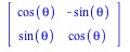
1. What familiar geometric transformation is P? Input P into Maple. How about MatrixInverse(P)?
2. Notice that the determinant of P is 1, so if we set up the system Px=0, the only solution would be the trivial solution. Hence the columns of P are linearly independent and so A is diagonalizable. Form
   A:=Matrix([[(cos(theta))^2,cos(theta)*sin(theta)],[cos(theta)*sin(theta),((sin(theta))^2)]]);
   
   Diag:=simplify(MatrixInverse(P).A.P)
   
   What familiar geometric transformation is Diag?
   
   
3. Notice that P.Diag.MatrixInverse(P) = A by matrix algebra and # 6. Writing out a transformation in terms of a P, the inverse of P, and a diagonal matrix will prove very useful in computer graphics, as we will see in the next couple of weeks. Fill in the blanks below. Recall that we read matrix composition from right to left.
   
   P.Diag.MatrixInverse(P) = A
   If we want to project a vector onto the y=tan(theta) x line, first we can perform MatrixInverse(P) which takes a vector and rotates it ___________________ by theta. Next we perform Diag, which projects onto the line _____________ . And finally we perform P, which rotates ___________________ by theta.
   
   It is sometimes easier to visualize by using a point on the y=tan(theta) x line, which we know is fixed under the projection. So take the vector (cos(theta),sin(theta)). Use matrix multiplication in Maple or geometric intuition to fill in these blanks: MatrixInverse(P) takes this point to the point ________________. Next we perform Diag which gives us the point _______________. Finally, we perform P, which takes the point back where we started to (cos(theta),sin(theta)).

   ---

4. Enter the matrix with columns (c,0) and (0,c) into Maple.
   Part A: Execute the Eigenvectors command.
   Part B: Let the matrix act on a column vector (x,y) via matrix multiplication.
   Part C: How does this transformation act on R²?
   Part D: Use Part C to explain your output in Part A.

   ---

5. Execute
   Sh:=Matrix([[1,k],[0,1]]);
   Part A: Execute the Eigenvectors command.
   Part B: Let the matrix act on a column vector (x,y) via matrix multiplication.
   Part C: Test out the image of a square with vertices (1,0), (1,1), (2,0), (2,1). What does Sh do to this square for k = 1? For k=2?
   Part D: How does Sh act as a transformation on R² for positive k values?
   Part E: Use Part D to explain your output in Part A.
   Part F: Is A diagonalizable? Why or why not?
   Part G: If k=0, Maple's response to Part A and your response to Part F are both incorrect - what should the responses be?

   ---

6. Execute
   Sv:=Matrix([[1,0],[k,1]]);
   Repeat Parts A, B, D, and E for this matrix.

   ---

7. Execute
   R:=Matrix([[cos(theta), sin(theta)],[sin(theta), -cos(theta)]]);
   Notice the difference between this matrix and P in #1 above.
   Part A: Apply the Eigenvectors(R); and Eigenvalues(R); commands. Notice that Maple will not output the eigenvectors, but it will output the eigenvalues.
   Part B: When theta=0, what geometric transformation is R? What are the eigenvectors for each eigenvalue in this case?
   Part C: When theta=Pi/2, what geometric transformation is R? What are the eigenvectors for each eigenvalue in this case?
   Part D: When theta=Pi, what geometric transformation is R? What are the eigenvectors for each eigenvalue in this case?
   Part E: What is the relationship between theta and the geometric transformation R(theta)?
   Part F: What are the eigenvectors for each eigenvalue for a general theta (hint: the reasoning and trigonometry is similar to what we used in the projection matrix questions.
   Part G: Is R(theta) diagonalizable?