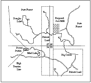
The Otsego Electric Company must run a power line from Power Station 23 in Section 34 to the saw mill under construction in Section 26. The saw mill is 2.3 km north and 5.2 km east of the power station; the intervening private land is 1,300 m wide (east-west). The power line must cross private land. The cost of an easement is $0.75 per meter through the state forest and $2.25 per meter on the private land.Determine the minimum cost route from the power station to the saw mill. Find the optimal size of the wire. Finally, determine the total cost of the wire for the route.
Project Report
There are three stages to the solution of this problem.
-
AWG Cost ($/m) Area (mcm) 000 0.25 167 - (AWG is American Wire Gauge,)
- (mcm is Millicircular mills.)
- (AWG is American Wire Gauge,)
- Using the data of the preceding table, find the constant of variation
and an equation for C_purch.
According to the theory of electricity, the resistance of the wire causes a power loss due to energy dissipation in the form of heat. The cost per meter of this loss, C_heat, is inversely proportional to the cross section area of the wire, A. From tests run by Otsego's Engineering Department, the following data are known:
-
AWG Cost ($/m) Area (mcm) 00 0.2385 105
-
- Using the values in the chart above, find the constant of variation and
an equation for C_heat.
- Take the cost per meter to be
C := A -> C_purch + C_heat
and find the cross section, A_min, in mcm, that minimizes cost and find the minimum cost C(A_min).Stage II. Determine the minimum cost path and its length.
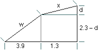
We begin the solution by taking the relevant data from the map and the description. Abstract from the physical situation to a mathematical model as shown in the next figure. (Be careful of your units.)Let x be the distance on private land and let w be the distance through the state forest, both measured in meters. Then, the cost of easement equation is
C_ease := $0.75 w + $2.25 x - Using the diagram above, express w in terms of x. Then minimize the
cost of easement with respect to x. With the value of x that gives the
minimum cost, find w and the total length,
L := w + x.Before invoking fsolve to find the critical points of C_ease as a function of x, examine a plot of C_ease over the x domain 1300..3600 (why this domain?) to determine the approximate coordinates of the minimum. Giving fsolve a sensible search interval may greatly speed your computations and, in some instances, is necessary.
Once we have found the distance d meters in the diagram above, we can plot the path of the power line as follows. We use d := 200 meters. It's not the correct answer! It's just for illustration.
d := 200:
Line := [0, 0], [3.9, 2.3 - d/1000], [5.2, 2.3];
Connect back to the origin to show the straight path, too.
Line := Line, [0, 0]:
Enter the following plot command to see the path.
plot([Line], x=0..6, y=-1..3, title=`Minimum Cost Path`);
Stage III. Calculate the total cost of the power line.
Combine the results of Stages I and II to find the total cost by using the formula
C_Total := C(A_min) * L + C_ease - Calculate the minimum total cost.
Stage I. Minimize the cost per meter related to the size of the wire.
The purchase cost per meter, C_purch, varies directly with the size of the wire --- i.e., with the amount of copper used per unit of cross section area A. The Purchasing Department has provided the figures:
Extension
After you submit your estimate, the supervisor tells you that you are responsible for the cost of the poles. The best estimate you can get is that they will cost between $120 and $130 a piece. What effect does adding the cost of poles have on your path?Report Requirements
Address your project report to your supervisor Leslie Fusaro. A minimal project report will include:- Answers with justifying narratives for 1 through 5.
- A Maple plot of the minimum path you have found.
Go to: Project Description.
Last update: Nov 12, 1995 (WmCB)

