Keeping a Race Track on a Car - Adapted from a Visual Linear Algebra (VLA) Module by Eugene A. Herman and Michael D. Pepe 

>	with(LinearAlgebra): with(plots): with(VLA):

 

If we want to create a realistic animation of a car moving along a curved road, we face two problems: 

• How can we keep the car on the road as the road curves?

• How can we keep the car pointing in the direction of motion?

We address these problems one at a time in what follows. 

Staying on the Curve 

Here is the parametrized curve we will use:  

>	x := t -> cos(t); y := t -> sin(2*t);

 

And here is the definition of the car in homogeneous coordinates: 

>	car := Matrix([[.15,-.15,-.15,.15],[0,.075,-.075,0],[1,1,1,1]]);

 

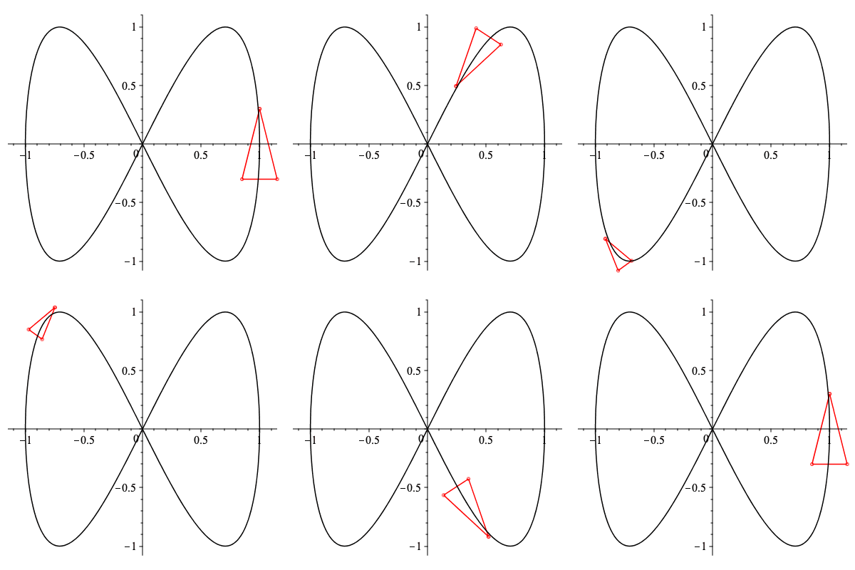
We draw the curve and the car in a single plot at t=0 on the curve. Note that the car is pointing in the direction of the positive x axis.  

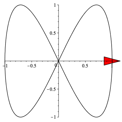
To create the illusion of motion along the curve, we need to place the car at numerous points along the curve.    

To keep the car on the curve, we translate the car from the origin to the curve using left multiplication - ie we perform Tcurve.car 

>	Tcurve := Matrix([[1, 0, cos(t)], [0, 1, sin(2*t)], [0, 0, 1]]);

 

(1)

 

>	Tcurve.car;

 

(2)

 

For example, let's plug in : 

>	T := Matrix([[1, 0, cos(1)], [0, 1, sin(2)], [0, 0, 1]]);

 

>

T.car;

 

>	carpict:=polygonplot([[0.15+cos(1),sin(2)],[-.15+cos(1),.075+sin(2)],[-.15+cos(1),-.075+sin(2)],[.15+cos(1),sin(2)]],color=red): display([carpict,pathpic]);

 

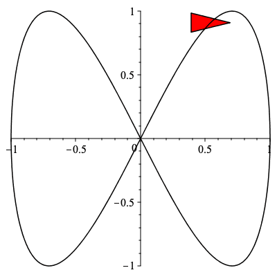Next, we can create a loop to create and save a similar plot for 33 values of t, ranging from to in increments of /16.  

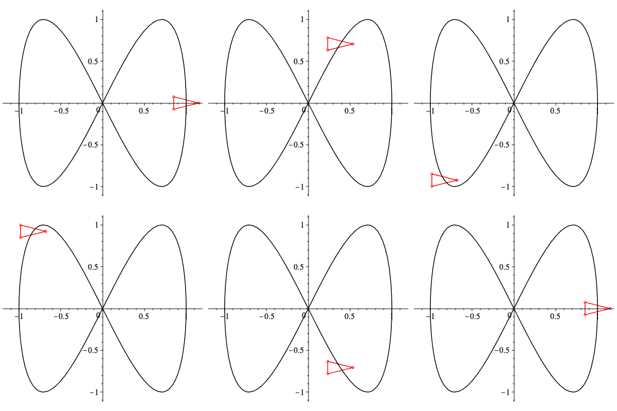Here's what I actually plotted, but it looks like (relatively) smooth motion to your eyes: 

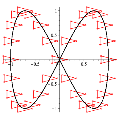
Pointing in the Direction of Motion 

We are halfway there!  Now to keep the car pointing in the direction of motion, we should rotate the car at each step of the animation. If we can find the appropriate rotation matrix R for each value of t, we will have solved our last remaining problem. 

Recall that the velocity (or tangent) vector to the parametrized curve always points in the direction of motion. We calculate the velocity vector by taking the derivative of each of the component functions of the curve with respect to t:  

>	vel := Vector([diff(x(t),t),diff(y(t),t)]);

 

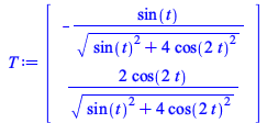
Next we define the unit vector T in the direction of vel, namely   by using the Pythagorean Theorem, or equivalently the square root of the dot product, to divide by the length of the vector by its norm: 

>	T := Vector[column]([[-sin(t)/(sin(t)^2+4*cos(2*t)^2)^(1/2)], [2*cos(2*t)/(sin(t)^2+4*cos(2*t)^2)^(1/2)]]);

 

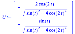
Notice that the columns of a 2 by 2 matrix transformation are the images of the standard unit vectors (1,0)  and . Since the car points in the direction of and we want it to point in the direction of the unit vector T, the image of must be T. Furthermore, if we were to rotate by 90 degrees counter-clockwise, we would get ; so rotating T by 90 degrees counter-clockwise, we get the image of . Let's call this image U. (It is the unit normal vector.) 

>	U := Vector[column]([[-2*cos(2*t)/(sin(t)^2+4*cos(2*t)^2)^(1/2)], [-sin(t)/(sin(t)^2+4*cos(2*t)^2)^(1/2)]]);

 

The rotation matrix we seek has columns T and U which are orthonormal vectors - ie unit length and orthogonal/perpendicular. 

>	R := Matrix([T,U]);

 

We must also construct the corresponding homogeneous version of R: 

>	Rh := Matrix([[-sin(t)/(sin(t)^2+4*cos(2*t)^2)^(1/2), -2*cos(2*t)/(sin(t)^2+4*cos(2*t)^2)^(1/2), 0], [2*cos(2*t)/(sin(t)^2+4*cos(2*t)^2)^(1/2), -sin(t)/(sin(t)^2+4*cos(2*t)^2)^(1/2), 0], [0, 0, 1]]);

 

>

 

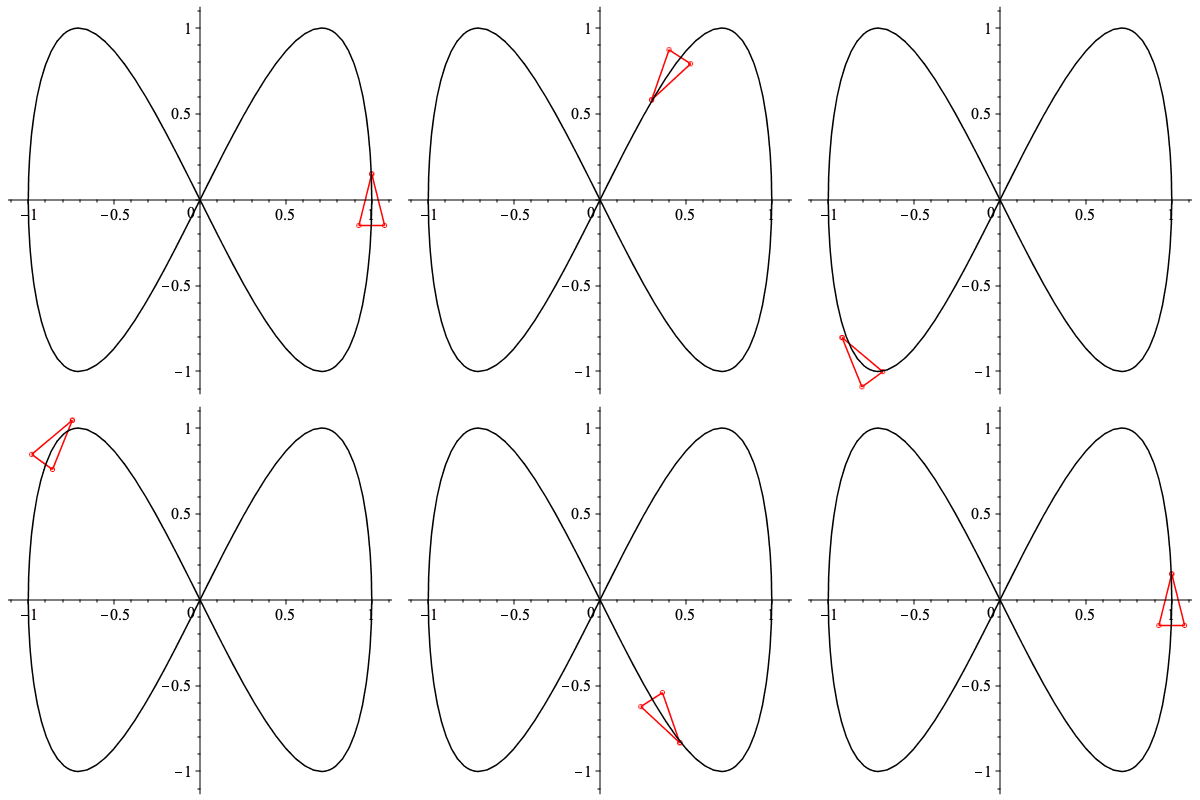
We are ready to test our results - we rotate the car at the origin and then translate it to the curve for various t values:  Tcurve.Rh.car (as is typical, order is important here, because we want to turn the steering wheel to point in the direction of the road before we start traveling!) 

Now try out the animation: 

Here is what happens if I mess up the order and use Rh.Tcurve.car rather than the correct Tcurve.Rh.car  

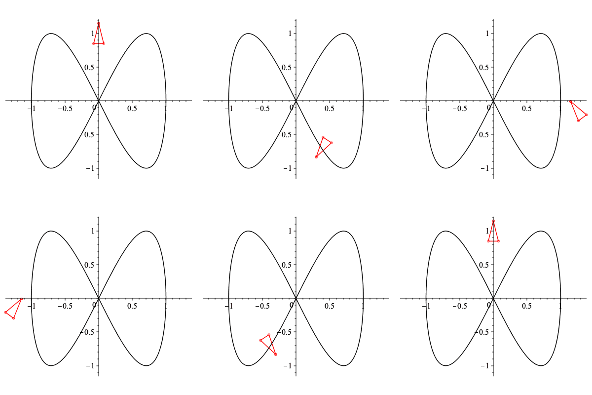
Tcurve.Rh.car is correct if we want to stay on the road. 

Why did we need to use the unit vectors in the rotation matrix?  Othewise that matix won't preserve distance, ie the size of the car.  

Let's see that in action by using the matrix obtained by the velocity vector (tangent) and a vector orthogonal to it (negative reciprocal slope) placed into homogeneous coordinates without diving by the norm: 

>