2240 Class Highlights
Fri June 21 Final research sessions. Course evaluations.
Upper level courses I teach include
Differential Geometry MAT 4140, Senior Capstone MAT 4040,
Instructional Assistant MAT 3520
Thur June 20 Tape up all components of the project.
Divide up the research session. Begin session 1. If time remains then
begin session 2. Mention test 3 revisions. Final research sessions.
Wed June 19 Test 3.
Review:
How are addition and scalar multiplication important in linear algebra?
What are some topics where we've seen algebra and geometry perspectives
Why do you think critical analysis and reasoning are a focus in this
course?
What are applications we've seen?
Work on the research presentations.
Tues June 18
We have been investigating applications of chapter 5 material to
mathematical biology. We'll finish the semester by
looking (briefly) at
applications of eigenvalues and eigenvectors to computer science and
physics:
Computer Graphics: Look at MatrixInverse(P).A.P,
which has the eigenvalues on the diagonal - definition of similarity,
like in 6.1 in the book.
Execute in Maple:
A:=Matrix([[(cos(theta))^2,cos(theta)*sin(theta)],[cos(theta)*sin(theta),
((sin(theta))^2)]]);
h,P:=Eigenvectors(A)
Diag:=simplify(MatrixInverse(P).A.P);
What geometric transformation is Diag?
Notice that P.Diag.MatrixInverse(P) = A by matrix algebra.
Writing out a transformation in terms of a P, the inverse of P, and a
diagonal matrix is very useful in computer graphics
[Recall that we read matrix composition from right to left].
Geometric intuition of
P.Diag.MatrixInverse(P) = A
If we want to project a vector onto the y=tan(theta) x line,
first we can perform MatrixInverse(P) which takes a vector and rotates it
counterclockwise by theta. Next we perform Diag,
which projects onto the x-axis, and finally we perform P, which rotates
clockwise by theta
Linear Transformations
Mathematical Physics:
heat diffusion
(48 seconds)
Eigenfunctions and the heat equation
Mention the spectrum of the Laplacian [divergence of
gradient] (the discrete sequence of eigenvalues). Spectrum is applied
to graphs, the heat equation,...
Can you hear the shape of a drum?
Sound of quantum
drums
END OF MATERIAL FOR TEST 3
Take any questions on test revisions, test 3
or the Final Research sessions
Chap 5 clicker questions#4-8
Mon June 17
Take any questions.
Finish the dynamical systems demo. Compute the eigenvalues using
determinant(A-lambdaI)=0
Clicker review of 2.8, 5.1 and 5.6:
#1, 5-8 in 2.8 clicker questions.
Chap 5 clicker questions#1 and #3
Fri June 14
Review eigenvalues and eigenvectors [Ax=lambdax, vectors that are scaled on
the same line through the origin, matrix multiplication is turned into scalar
multiplication]. Solving Ax=lambdax algebraically using
determinant(A-lambdaI)x=0, and substituting each lambda in to find a
basis for the eigenspaces of A and equivalently the nullspace of (A-lambda I).
Geometry of Eigenvectors and compare
with Maple.
Eigenvector decomposition for a diagonalizable matrix A_nxn [where the
eigenvectors form a basis for all of Rn]
Foxes and Rabbits demo on ASULearn
Dynamical Systems and Eigenvectors on ASULearn
If ___ equals 0 then we die off along the line____ [corresponding to
the eigenvector____], and in all other cases we [choose one: die off or grow or
hit and then stayed fixed] along the line____ [corresponding to the
eigenvector____].
Thur June 13
clicker questions
on inverses and determinants #3-4 and 6-8
Review and finish 2.8 using the matrix 123,456,789 and finding the
Nullspace and ColumnSpace (using 2 methods - reducing the spanning equation
with a vector of b1...bn, and separately by examining the pivots of the
ORIGINAL matrix.)
Define eigenvalues and eigenvectors [Ax=lambdax, vectors that are scaled on
the same line through the origin, matrix multiplication is turned into scalar
multiplication].
Eigenvectors of Matrix([[0,0],[1,0]]);
Algebra: Show that we can solve using det(A-lambdaI)=0 and (A-lambdaI)x=0.
Compute the eigenvectors of Matrix([[0,1],[1,0]] by-hand and compare with
Maple's work.
Wed Jun 12 Test 2 until 11:35.
Begin 2.8 in order to lead to eigenvalues and applications
(2.8, 4.9 and 5.1, 5.2, 5.3 and 5.6 selections, 7.1 as time allows).
Tues Jun 11
Review the 2 determinant methods for the 123,456,789 matrix.
Show that for 4x4 matrix in Maple, only Laplace's method will work.
The connection of row operations to determinants
clicker questions on inverses and
determinants #3-5
Continue determinant work via the relationship of row operations
to the geometry of determinants via a demo on ASULearn.
Show that det A non-zero can be
added into Theorem 8 in Chapter 2.
Algebraic and geometric ideas related
to the determinant, including the determinant of A inverse, A transpose and
A triangular (such as in Gaussian form).
Mon Jun 10
2.3 and linear transformation
Clicker questions #8-9
End of Computer Graphics Demo - rotating a 3-d object.
Computer graphics continued, including the benefit of derivatives and
unit length vectors in keeping a car on a race track - demo on ASULearn.
Discuss Yoda via the file yoda2.mw with
data from Lucasfilm LTD as on
Tim's Page which
has the data.
Begin chapter 3 via mentioning google searches:
application of determinants in physics
application of determinants in economics
application of determinants in chemistry
application of determinants in computer science
Eight queens and determinants
Chapter 3 in Maple via MatrixInverse
command for 2x2 and 3x3 matrices and then determinant work, including 2x2
and 3x3 diagonals methods, and Laplace's expansion (1772 - expanding on
Vandermonde's method) method in general. [general history dates to
Chinese and Leibniz]
Fri Jun 7
2.3 and
linear transformation Clicker questions #1-7
general geometric transformations on
R2 [1.8, 1.9]
Computer graphics Demo on ASULearn [2.7]
Thur Jun 6
A_mxn (not square). Can Ax=0 have only the trivial soluiton
a) No that statement is impossible
b) Yes when the columns of A are l.i.
c) Yes when the columns of A are l.i. and A has m pivot rows
d) Yes when the columns of A are l.i. and A has n pivot columns
e) Both c and d
Review
guidelines for Problem Sets, including
You have more
time to work on fewer problems than practice exercises - Maple,
interesting applications...
Counterexamples for false
statements [If A then B counterexample: A is true but the conclusion
B is false]
Print Maple or show by-hand work
Annotated work / explanations that show your critical reasoning
In 2.3 # 12, in the instructions before 11, A is given as nxn
In the Condition Number problem, be careful of my additional
instructions (inverse method with fractions...)
Computer graphics and linear transformations (1.8, 1.9, 2.3 and 2.7)
Begin with dilations
Guess the transformation on ASULearn
Revisit Theorem 8 in 2.3 by incorporating the
language of linear transformations [while also covering 1-1 and onto material
in 1.9]
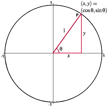
Review the unit circle
Wed Jun 5
2.3 clicker questions
2.2 and 2.3 clicker questions
Theorem 8 in 2.3 [without linear transformations]
Catalog description: A study of vectors, matrices and linear
transformations, principally in two and three dimensions,
including
treatments of systems of linear equations, determinants,
and
eigenvalues.
-2.1-2.3 Applications: Coding, Condition Number and Linear
Transformations (2.3, 1.8, 1.9 and 2.7)
-Chapter 3 determinants and applications
-Eigenvalues and applications (2.8, 4.9 and chap 5 selections,
7.1... as time allows)
-Final research
sessions [research a topic related to the course that you are
interested in]
Hill Cipher
| A |
B |
C |
D |
E |
F |
G |
H |
I |
J |
K |
L |
M |
N |
O |
P |
Q |
R |
S |
T |
U |
V |
W |
X |
Y |
Z |
| 1 |
2 |
3 |
4 |
5 |
6 |
7 |
8 |
9 |
10 |
11 |
12 |
13 |
14 |
15 |
16 |
17 |
18 |
19 |
20 |
21 |
22 |
23 |
24 |
25 |
26 |
Condition # of matrices
Maple file on Coding and Condition Number and
PDF version
Tues Jun 4
Continue via 2.1 clicker questions #7-8
and 10
Go over the last 2 problems on the practice set: 21 and 23:
last col AB is all 0 but B has no col of 0s. [... A.lastcolB]
CA=I. Apply to Ax=0 and reason why A cannot have more columns than rows.
Inverse of a matrix.
twobytwo := Matrix([[a, b], [c, d]]);
MatrixInverse(twobytwo);
three := Matrix([[a, b, c], [d, e, f], [g, h, i]]);
Introduction to Linear maps
scalerow3 := Matrix([[1, 0, 0], [0, 5, 0], [0, 0, 1]]);
scalerow3.three;
swaprows13 := Matrix([[0, 0, 1], [0, 1, 0], [1, 0, 0]]);
swaprows13.three;
usualrowop := Matrix([[1, 0, 0], [0, 1, 0], [-2, 0, 1]]);
usualrowop.three;
The black hole matrix: maps R^2 into the plan but not onto (the range
is the 0 vector).
Finish 2.2 and work on 2.3: A matrix has a unique inverse, if it exists.
A matrix with an inverse has Ax=b with unique solution x=A^(-1)b, and then
the columns span and are l.i...
Repeated methodology: apply inverse, use associativity, use def of inverse
to obtain the Identity, use definition of Identity to cancel it.
Mon Jun 3 Test 1 from 10:20-11:35 and then we resume class.
If you finish early you may leave and come back then.
Matrix algebra
Continue with 2.1 and 2.2. Transpose of a matrix via Wikipedia,
including Arthur Cayley. Applications including least squares estimates,
such as in linear
regression, data given as rows (like Yoda).
Continue via 2.1 clicker questions #9
Fri May 31
Continue via 2.1 clicker questions 5-6
Powerpoint file.
Matrix multiplication
Algebra of matrix multiplication: AB and BA...
Thur May 30 Take any questions.
#5 onward on
Chap 1 review clicker questions
Review #4: (a: v2 = 4v2. b: v3= -v1 + 2v2 c: v1 + v2 = v3).
End of Material for Test 1
Image 1
Image 2
Image 3
Image 4
Image 5
Image 6
Image 7.
Continue via 2.1 clicker questions 1-4
Wed May 29 Take any questions.
Problem Set 2 clicker questions
Chap 1 review clicker questions #1-4
Tues May 28
Review definitions
and the algebra and geometry of in the span (ie is a linear
combination, the span, and l.i.)
Maple Code:
M:=Matrix([[1, 4, 7, 5], [2, 5, 8, 7], [3, 6, 9, 9]]);
ReducedRowEchelonForm(M);
M:=Matrix([[1, 4, 7, 5], [2, 5, 8, 7], [3, 6, 9, 10]]);
ReducedRowEchelonForm(M);
Span1:=Matrix([[1, 4, 7, 5,b1], [2, 5, 8,7,b2], [3, 6, 9,9,b3]]);
Span2:=Matrix([[1, 4, 7, 5,b1], [2, 5, 8,7,b2], [3, 6, 9,10,b3]]);
li1:= Matrix([[1, 4, 7, 5,0], [2, 5, 8,7,0], [3, 6, 9,9,0]]);
li2:= Matrix([[1, 4, 7, 5,0], [2, 5, 8,7,0], [3, 6, 9,10,0]]);
li3:= Matrix([[1, 4, 5,0], [2, 5,7,0], [3, 6,10,0]]);
a1:=spacecurve({[t, 4*t, 7*t, t = 0 .. 1]}, color = red, thickness = 2):
a2:=textplot3d([1, 4, 7, ` vector [1,4,7]`], color = black):
b1:=spacecurve({[2*t,5*t,8*t,t = 0 .. 1]}, color = green, thickness = 2):
b2:=textplot3d([2, 5, 8, ` vector [2,5,8]`], color = black):
c1:=spacecurve({[3*t, 6*t, 9*t, t = 0 .. 1]},color=magenta,thickness = 2):
c2:=textplot3d([3,6,9,`vector[3,6,9]`],color = black):
d1:=spacecurve({[0*t,0*t,0*t,t = 0 .. 1]},color=yellow,thickness = 2):
d2:=textplot3d([0,0,0,` vector [0,0,0]`], color = black):
e1 := spacecurve({[3*t, 6*t, 10*t, t = 0 .. 1]},color=black,thickness = 2):
display(a1, a2, b1, b2, c1, c2, d1, d2,e1);
In R^3, span but not l.i., l.i. but not span, both l.i. and span.
Coffee mixing clicker question
The matrix vector equation and the augmented matrix.
Decimals (don't use in Maple) and fractions, and the connection of
mixing to span and linear combinations. Geometry of the columns as a plane
in R^4, of the rows as 4 lines in R^2 intersecting in the point (40,60)
Mon May 27
Take questions. Review
linear combination and span.
Ax via using weights from x for columns of A versus
Ax via dot products of rows of A with x
and Ax=b the same (using definition 1 of linear combinations of the columns)
as the augmented matrix [A |b]
Finish theorem 4 in 1.4.
1.5: vector parametrization equations of homogeneous and
non-homogeneous equations.
definitions
Span: represent. Linearly Independent: efficiency. Basis: both.
In R^2, span but not li, li but not span, li plus span.
Fri May 24 Review linear combination language (addition and
scalar multiplication of vectors).
1.3 clicker questions 1, 2 and 4
and introduce the algebra and geometry of span and linear combinations.
1.4.
Thur May 23
1.1 and 1.2 clickers #4 onward
History of linear equations and the term "linear algebra"
images, including the Babylonians 2x2 linear
equations, the
Chinese 3x3 column elimination method over 2000 years ago, Gauss' general
method arising from geodesy and least squares methods for celestial
computations, and Wilhelm Jordan's contributions.
Gauss quotation. Gauss was also involved in
other linear algebra, including the
history of vectors, another important "linear" object.
vectors, scalar mult and addition, linear combinations and weights,
vector equations and connection to 1.1 and 1.2 systems of equations and
augmented matrix
Wed May 22
Register the i-clickers
Review vocabulary from day 1 or the hw readings
Elimination
We already saw examples of augmented matrices with 0
solutions, via parallel planes, as well as 3 planes that just don't
intersect concurrently:
implicitplot3d({x-2*y+z-2, x+y-2*z-3, (-2)*x+y+z-1}, x = -4 .. 4,
y = -4 .. 4, z = -4 .. 4)
implicitplot3d({x+y+z-3, x+y+z-2, x+y+z-1}, x = -4 .. 4, y = -4 .. 4,
z = -4 .. 4)
Terminology and Idea:
Systems of equations. Unknowns. Coefficients.
Solutions.
Augmented matrix. Pivots.
Algebraic Parametrization. Geometric Plot. Points. Lines.
Planes. Gaussian (Echelon) and Gauss-Jordan
(ReducedRowEchelon). Homogeneous system. Trivial solution.
1.1 and 1.2 clickers #1-3
Tues May 21
Fill out the information sheet
and work on the introduction to linear algebra handout motivated from
Evelyn Boyd Granville's favorite
problem.
Slide
At the same time, begin 1.1 and 1.2 including geometric perspectives,
by-hand algebraic Gaussian Elimination and pivots,
solutions,
plotting and geometry, parametrization and GaussianElimination in Maple.
In addition, do #5 with
k as an unknown but constant coefficient. Prove using geometry of lines
that the
number of solutions of a system
with 2 equations and 2 unknowns is 0, 1 or infinite.
Look at the geometry using implicitplot3d,
number of missing pivots, and parametrization of x+y+z=1.
Algebraic and geometric perspectives in 3-D and solving using by-hand
elimination, and ReducedRowEchelon and
GaussianElimination.
3 equations 2 unknowns with one solution in the plane R2,
3 equations 3 unknowns with infinite solutions, one solution and no
solutions in R3.
Mention homework and the class webpages