2240 class highlights

Wed Dec 12 9-11:30am final research sessions

Thur Dec 6 Computer graphics continued, including the benefit of derivatives and unit length vectors in keeping a race track on a curve.
Discuss Yoda via the file yoda2.mw with data from Lucasfilm LTD as on Tim's Page which has the data.
Final project topics and assign sessions
Evaluations

Tues Dec 4 Continue transformations Begin computer graphics demo via definition of triangle := Matrix([[4,4,6,4],[3,9,3,3],[1,1,1,1]]); and then ASULearn Computer Graphics Example D and the usefulness of transformations like Tinverse.R.T. Look at Homogeneous 3D coordinates and Example G. Then Example I, keeping an object along a curve. If time remains, show twister, the movie and keeping a race track on a curve.

Thur Nov 29 Test 3 with Dr. Thomley while I am speaking in Chicago.

Tues Nov 27 Take questions
If the column vector a=Matrix([[a1],[a2],...,,[an]]) is a nontrivial eigenvector for A, as outputed by Maple, then A has at least the eigenvectors as follows:
a) all of Rⁿ
b) an entire line through the origin in Rⁿ
c) just a and the 0 vector
d) just a
e) a and a second vector b that Maple outputs

If a matrix A has repeated eigenvalues then
a) A is diagonalizable
b) A is not diagonalizable
c) We cannot tell whether A is diagonalizable yet

Finish reflection on: Linear Transformations: Chap 6 and review the eigenvectors/eigenvalues.
Mention Rural and Urban Populations and stability Last few examples in the Dynamical systems demo on ASULearn, begining with the dynamic graph of various intitial conditions and continuing.

We did not have time to get to Chapter 7 review

Tues Nov 20

Clicker review of the problem set: Is Matrix([[1,k],[0,1]]) diagonalizable?
a) yes
b) no

Given a square matrix A, to solve for eigenvalues and eigenvectors
a) (lambdaI - A)x=0 is equivalent, so, since we are looking for nontrivial x solutions, that means that this homogeneous system must have infinite solutions, so we can solve for det(lambdaI- A)=0 via the theorem in Chapter 3.
b) Once we have a lambda that works, we can take the inverse of (lambdaI- A) to solve for the eigenvectors
c) Once we have a lambda that works, we can create the augmented matrix [lambdaI- A|0] and reduce to solve for solutions and write out a basis.
d) a and b
e) a and c

How many non-trivial real eigenvectors does Matrix([[cos(pi),-sin(pi)],[sin(pi),cos(pi)]]) have?
a) 0
b) 1
c) 2
d) infinite
e) none of the above

How many linearly independent eigenvectors does Matrix([[cos(pi),-sin(pi)],[sin(pi),cos(pi)]]) have?
a) 0
b) 1
c) 2
d) infinite
e) none of the above

Is Matrix([[cos(pi),-sin(pi)],[sin(pi),cos(pi)]]) diagonalizable?
a) yes
b) no

How many nontrivial real eigenvectors does Matrix([[cos(pi/2),-sin(pi/2)],[sin(pi/2),cos(pi/2)]]) have
a) 0
b) 1
c) 2
d) infinite
e) none of the above

Linear Transformations: Chap 6 and review the eigenvectors/eigenvalues.
Show that a rotation matrix rotates algebraically as well as geometrically. Discuss rotation, shear, dilation and projection.
For projection, first review the unit circle
execute:
A:=Matrix([[(cos(theta))^2,cos(theta)*sin(theta)],[cos(theta)*sin(theta), ((sin(theta))^2)]]);
h,P:=Eigenvectors(A)
Diag:=simplify(MatrixInverse(P).A.P);
What geometric transformation is Diag?
Notice that P.Diag.MatrixInverse(P) = A by matrix algebra. Writing out a transformation in terms of a P, the inverse of P, and a diagonal matrix will prove very useful in computer graphics [Recall that we read matrix composition from right to left].
Geometric intuition of P.Diag.MatrixInverse(P) = A If we want to project a vector onto the y=tan(theta) x line, first we can perform MatrixInverse(P) which takes a vector and rotates it counterclockwise by theta. Next we perform Diag, which projects onto the x-axis, and finally we perform P, which rotates clockwise by theta
Build up intuition for transformations and part 2.

Thur Nov 15 Clicker review: How many linearly independent eigenvectors does Matrix([[1,2],[2,1]]) have?
a) 0
b) 1
c) 2
d) infinite
e) none of the above

How many eigenvectors does Matrix([[1,2],[2,1]]) have?
a) 0
b) 1
c) 2
d) infinite
e) none of the above

An eigenvector allows us to turn:
a) Matrix multiplication into matrix addition
b) Matrix addition into matrix multiplication
c) Matrix multiplication into scalar multiplication
d) Matrix addition into scalar multiplication
e) none of the above

Explain why the eigenvectors of Matrix([[1,2],[2,1]]) satisfy the definitions of span and li by setting up the corresponding equations and solving.
li :=
span:=
Also do to see that MatrixInverse(P).A.P has the eigenvalues on the diagonal - definition of diagonalizability.

Derivation that for eigenvectors x for A, A^kx = lambda ^kx

Derivation that A P = P times the diagonal matrix of eigenvalues [which is how we showed that MatrixInverse(P).A.P = Diag]

Eigenvector decomposition for a diagonalizable matrix A
Finish the last 3 eigenvectors clicker questions.
Foxes and Rabbits demo on ASULearn. 7.2.

Tues Nov 13 Take questions on the eigenvector hw on the Healthy Sick worker problem from Problem Set 3. Begin 7.1 Define eigenvalues and eigenvectors [Ax=lambdax, vectors that are scaled on the same line through the origin, matrix multiplication is turned into scalar multiplication].
Prove that we can solve using det(lambdaI-A)=0 and (lambdaI-A)x=0
Compute the eigenvectors of Matrix([[0,1],[1,0]] by-hand and compare with Maple's work. Mention the book presenting the coefficient matrix instead of the augmented matrix for the system (lambdaI-A)x=0 [Ax=lambdax].
See where points that make up a square go: [0,0], [1,0], [0,1], [1,1] and then [-1,1]. What kind of geometric transformation is this?
Then compare with the Geometry of Eigenvectors to examine the type of geometric transformation.
We'll be working with rotations, reflections and projections, dilations, translations and shears here and in computer graphics.
Eigenvectors and eigenvalues of Matrix([[1,2],[2,1]) in Maple.
Begin eigenvectors clicker questions.

Thur Nov 8 Test 2

Tues Nov 6
Continue 4.5 clicker questions. Mention the ice cream mixing questions, which we will come back to if there is time.
Review the Healthy Sick worker problem from Problem Set 3. Begin 7.1 Define eigenvalues and eigenvectors [Ax=lambdax, vectors that are scaled on the same line through the origin, matrix multiplication is turned into scalar multiplication]. Examine Geometry of Eigenvectors
Take questions on the test.
chap 4 clicker review questions.
Finish 4.5 clicker questions.

Thur Nov 1
Take questions on 4.6 from hw readings as well as the file Span and Linear Independence comments from hw.
Definitions.
Prove that span + l.i. for a basis give a unique representation.
Begin 4.5 clicker questions

Tues Oct 30 *****SNOW DAY****
Look at Span and Linear Independence comments.
Definitions.
First 2 problem set questions - revisit using the language of span and li
Prove that span + l.i. for a basis give a unique representation.
4.6 and revisit problem set 1 questions in this context.
4.5 clicker questions

Thur Oct 25
Definitions. 4.4 clicker questions.
Revisit ps 4 numbers 1 and 2 in the language of span and l.i.
Are Vector([1,2,3]), Vector([0,1,2]), Vector([-2,0,1]) linearly independent?
Are Vector([1,2,3]), Vector([0,1,2]), Vector([-1,0,1]) linearly independent?
If not, what do they span geometrically and algebraically?
Maple work
Maple Code:
with(LinearAlgebra): with(plots):
a1:=spacecurve({[1*t,2*t,3*t,t=0..1]},color=red, thickness=2):
a2:=textplot3d([1,2,3, ` vector [1,2,3]`],color=black):
b1:=spacecurve({[0*t,1*t,2*t,t=0..1]},color=green, thickness=2):
b2:=textplot3d([0,1,2, ` vector [0,1,2]`],color=black):
c1:=spacecurve({[-2*t,0*t,1*t,t=0..1]},color=magenta, thickness=2):
c2:=textplot3d([-2,0,1, ` vector [-2,0,1]`],color=black):
d1:=spacecurve({[0*t,0*t,0*t,t=0..1]},color=yellow, thickness=2):
d2:=textplot3d([0,0,0, ` vector [0,0,0]`],color=black):
display(a1,a2, b1,b2,c1,c2,d1,d2);

Tues Oct 23

Rotation matrices using multiplication satisfying ax 1-5, but violating 6. Solutions to Ax=[1 2] column vectors. Begin 4.4 and 4.5: Representations of R^2 and R^3 under linear combinations - ie does a set of vectors span and if not, what linear space through the origin is the span? Definitions.
column vectors sets to test span (always inconsistent when augmenting with (x,y) or (x,y,z)):
(0,0)
(0,1) and (0,2)
(1,0), (0,1)
(1,0), (0,1), and (1,1)
(1,0,0), (0,1,0), and (0,0,1)
(1,4,7), (2,5,8), and (3,6,9)
(1,4,7), (2,5,8), and (3,7,9)
any set of 2 vectors in R^3
linear independence for (0,1) and (0,2)

Thur Oct 18 Continue 4.2 and 4.3.
x+y+z=0 in R^3.
a) satisfies both axiom 1 and 6
b) satisfies axiom 1 but not axiom 6
c) satisfies axiom 6 but not axiom 1
d) satisfies neither axiom 1 nor axiom 6

Continue generating vector spaces in R^2 and R^3 under linear combinations. A proof of the subspaces of R^3.

nxn matrices that have columns adding to 1
a) satisfies both axiom 1 and 6
b) satisfies axiom 1 but not axiom 6
c) satisfies axiom 6 but not axiom 1
d) satisfies neither axiom 1 nor axiom

The union of the lines y=x and y=-x [ie column vectors [x,y] that satisfy y=x or y=-x]
a) satisfies both axiom 1 and 6
b) satisfies axiom 1 but not axiom 6
c) satisfies axiom 6 but not axiom 1
d) satisfies neither axiom 1 nor axiom

Tues Oct 16
Review the language of linear combinations:
The vector x is a linear combination of the vectors v1,...,vn if
a) x can be written as a combination of addition and/or scalar multiplication of the vectors v1,...,vn
b) x is in the same geometric (and linear) space that the vectors v1,...,vn form under linear combinations (line, plane, R^3...)
c) both a and b
d) neither a nor b

Revisit the
1 2 3
4 5 6
7 8 9
determinant 0 matrix
with(LinearAlgebra):
with(plots):
col1 := spacecurve([t, 4*t, 7*t], t = 0 .. 1):
col2 := spacecurve([2*t, 5*t, 8*t], t = 0 .. 1):
col3 := spacecurve([3*t, 6*t, 9*t], t = 0 .. 1):
display(col1, col2, col3):
Then change the 6 to a 7 in the last column and discuss using the language of linear combinations, as well as the determinants

Begin 4.2 and 4.3, including solutions to y=3x+2 and y=3x in R^2. Look at a proof of all the subspaces of R^2.

Tues Oct 9 Clicker questions 4.1 Finish Geometry of determinants and row operations via demo on ASULearn. Linear combinations. Discuss what c1v1+c2v2=b could look like for various v1 and v2. Look at the resulting matrix equation: [v1 v2]c=b with v's as columns. The augmented matrix is [v1 v2|b]. Coffee Mixing as well as the geometry of the columns (chap 4) and the rows (chap 1) and numerical methods issue related to decimals versus fractions.

Thur Oct 4 Test 1

Tues Oct 2 Look at tu+v as vectors whose tips lie on the line that goes through the tip of v and is parallel to u. Revisit the proof that there are 0, 1 or infinite solutions to a linear system, and see that sol1 + t (sol1-sol2) is vectors whose tips end on the line connecting the tips of sol1 and sol2 [t=0 and t=-1 for example]. Geometry of determinants and row operations via demo on ASULearn. Take questions on Test 1.

Thur Sep 27 Continue with 3.3 derivations. Finish Chapter 3 clicker questions. Begin the algebra and geometry of column vectors: scalar multiplication and addition revisited, as well as the geometry.

Tues Sep 25 Continue determinant work via Laplace's expansion method and the relationship of row operations to determinants. Chapter 3 clicker questions.

Thur Sep 20
Finish Markov/stochastic/regular matrices.
Hill cipher using matrices
Patent Diagrams
Hill Cipher slides
Discuss regression line.
3.1-3.2: Begin Chapter 3 in Maple via MatrixInverse command for 2x2 and 3x3 matrices and then determinant work. Chapter 3 clicker questions

Tues Sep 18
chapter 2 clicker review
Begin 2.5: Applications of the algebra of matrices in 2.5:
Review:
Matrix Multiplication: profit (units must match up for this to be the case), rotation matrices in 2.1 #32 practice problems,
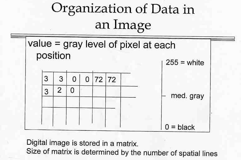
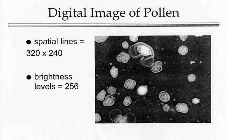
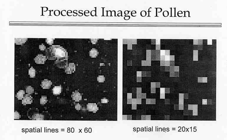
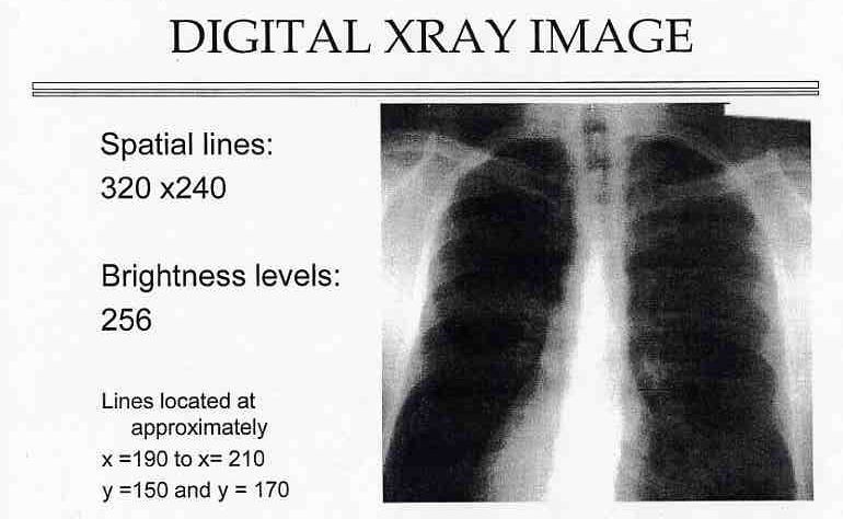
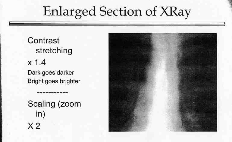
Matrix addition: adding digital images, adding sales month to month...
Scalar multiplication: scaling images, 1.2*J target sales for a 20% increase...
2.5:
2.5 clicker question.
Markov/stochastic/regular matrices.

Thur Sep 13
Finish 2.3:
Continue with the algebra of matrices.
Prove that in a linear system with n variables and n equations there may be 0, 1 or infinite solutions.

Tues Sep 11 Finish the 2.1 and 2.2 clicker questions

Review ps1 #5 (44 part d): If k=-6 then
a) there are no solutions
b) there is a unique solution
c) there is an entire line of solutions
d) there is an entire plane of solutions
e) I don't know

Review 2.1 #32 and that we will see these later as representing rotation matrices where A(alpha)*A(beta) = A(alpha +beta).

Review 2.2 #35 part c: To solve this problem....
a) We can set a, b, c=0. We know 0*matrix = matrix of all 0s, so when we add the three trivial (all 0s) column vectors together we obtain the trivial column vector, as desired.
b) We can leave a, b, c as general constants, like in the previous k problem, and then using matrix algebra we obtain a system of three equations in the three unknowns. We can create a corresponding matrix for the system and use Gauss-Jordan on it to show that (0,0,0) is the only solution for (a,b,c)
c) Both of the methods described in a) and b) work to solve this problem.
d) Neither of the methods work to answer the question.

Do 2.3.

Tues Sep 4
Begin with first few 2.1 and 2.2 clicker questions including matrix addition.
Image 1 Image 2 Image 3 Image 4 Image 5 Image 6 Image 7.
Powerpoint file.
Continue with the matrix multiplication clicker questions.

Thur Aug 30 Register remaining i-clickers. Go over text comments in Maple and distinguishing work as your own.

Which of the following are true regarding problem sets (like due on Tues):
a) I am only allowed to use the book, my group members, the math lab and Dr. Sarah for help on the problem set.
b) I can use any source for help, but the work and explanations must be distinguished as originating from my own group.
c) I must acknowledge any help, like "the idea for problem 1 came from discussions with johnny."
d) Both b) and c)
1.3 via the traffic problem and mention a circuit Gaussian review, which includes both same number of unknowns as variables as well as a different number of unknowns as variables.

Tues Aug 28 Register remaining i-clickers. Gauss quotation Go over 59 b and 73 from the hw. Discuss the Problem Set Guidelines, Write-Ups and hand out the Commands and Hints.
We already saw examples of matrices with 0 solutions, via parallel planes, as well as 3 planes that just don't intersect concurrently: implicitplot3d({x-2*y+z-2, x+y-2*z-3, (-2)*x+y+z-1}, x = -4 .. 4, y = -4 .. 4, z = -4 .. 4) implicitplot3d({x+y+z-3, x+y+z-2, x+y+z-1}, x = -4 .. 4, y = -4 .. 4, z = -4 .. 4)
Finish Questions.
In 3-D how many solutions to a linear system of equations are possible? What is the geometry? What is the Gaussian reduction?
How about a system that intersects in one point? Infinite solutions and parametrizations.

Thur Aug 23 Register i-clickers. Take questions on the syllabus and hw. History of linear equations and the term "linear algebra" images, including the Babylonians 2x2 linear equations, the Chinese 3x3 column elimination method over 2000 years ago, Gauss' general method arising from geodesy and least squares methods for celestial computations, and Wilhelm's contributions for
3 equations 2 unknowns with one solution. 3 equations 3 unknowns with infinite solutions.
Questions. Algebraic and geometric perspectives in 3-D and solving using by-hand elimination, and ReducedRowEchelon and GaussianElimination.

Tues Aug 21 Fill out the information sheet and work on the introduction to linear algebra handout motivated from Evelyn Boyd Granville's favorite problem. At the same time, begin 1.1 and 1.2 including geometric perspectives, by-hand algebraic Gaussian Elimination, solutions, plotting and geometry, parametrization and GaussianElimination in Maple. In addition, do #5 with k as an unknown but constant coefficient. Prove using geometry that the number of solutions of a system with 2 equations and 2 unknowns is 0, 1 or infinite.