2240 class highlights
Fri June 26 final research presentations
and peer and self-evaluations. Collect test 3 revisions.
Thur June 25 final research presentations
and peer evaluations
Wed June 24
Clicker question on interests
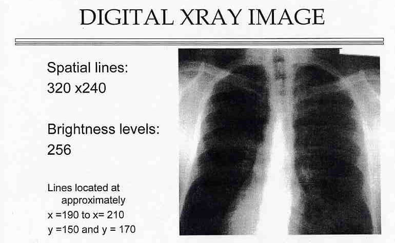
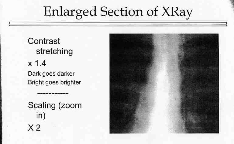
April was mathematics awareness month - the theme was magic, mystery and
mathematics.
Have the class give me a 3x3 matrix.
Look at
h,P:=Eigenvectors(A)
MatrixInverse(P).A.P
which (ta da) has the eigenvalues on the
diagonal
(when the columns of P form a basis for Rn)-diagonalizability.
[We can uncover the mystery
and apply this to computer
graphics].
Applications to mathematical physics,
quantum chemistry...
Share the final research presentations topic
(name, major(s), concentrations/minors, research project idea, and
whether you prefer to go 1st, 2nd or have no preference)
Last slide of final research presentations
evaluation
Tues Jun 22 Test 3. Use the remainder of class time to
work on the final research presentations.
Mon Jun 21
Big picture discussion
Review final research presentations
Clicker survey questions
Review for test 3 and take questions on
the study guide, material or final research
presentations
Fri Jun 18
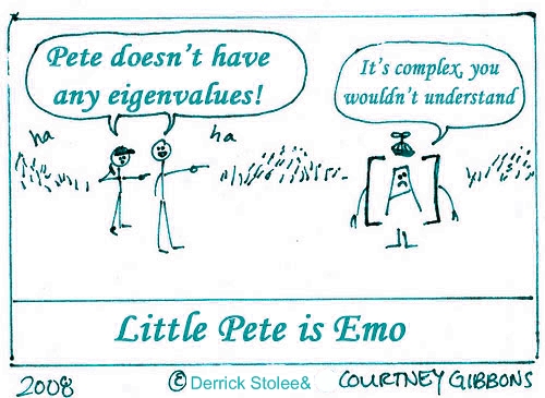
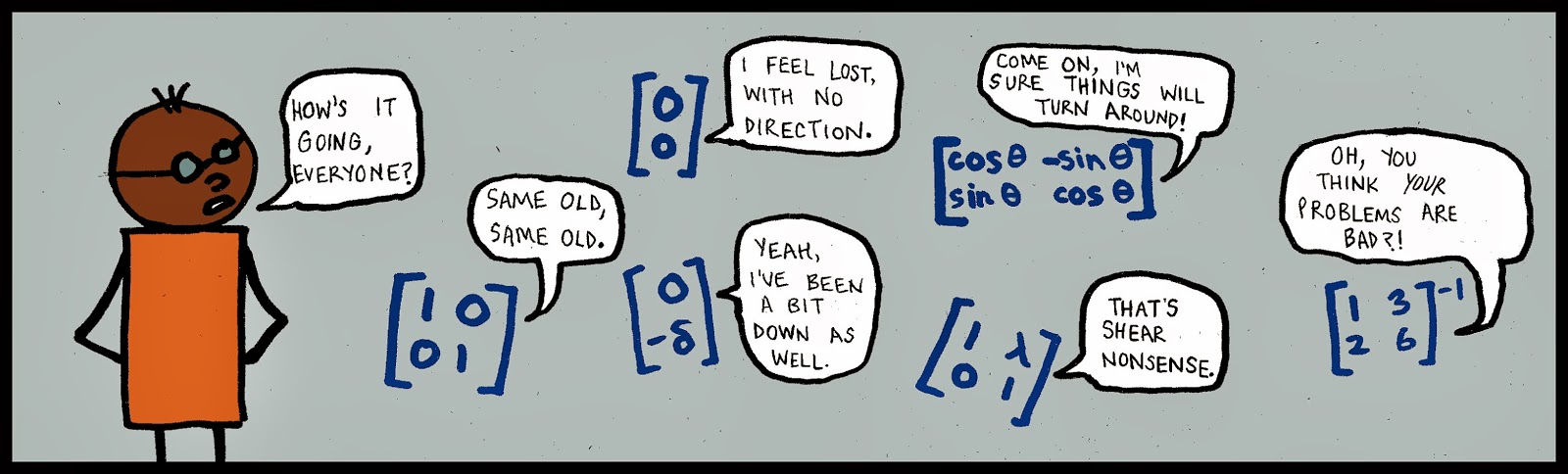
Eigenvector
comic 1, comic 2
Clicker questions---review of
eigenvectors #1-5
Clicker questions---
eigenvector decomposition (5.6) part 2 #1, 2 and 3
Dynamical Systems and
Eigenvectors remaining examples
Clicker questions---
eigenvector decomposition (5.6) part 2 #4-6
final research presentations
Hamburger earmuffs and the pickle matrix
Thur June 17
Review eigenvectors and eigenvalues:
definition (algebra and geometry)
What equations have we seen
Why we use det(A-lambdaI)=0
Why we use the eigenvector decomposition versus high powers of A for
longterm behavior (reliability)
Clicker questions in 5.1#1-3
Dynamical Systems and
Eigenvectors first example
Clicker questions on
eigenvector decomposition (5.6) part 1#1-4 [Solutions: 1. a), 2. c), 3. c), 4. b)]
Highlight predator prey, predator predator or cooperative systems
(where cooperation leads to sustainability)
Geometry of Eigenvectors and compare
with Maple
>Ex1:=Matrix([[0,1],[1,0]]);
>Eigenvalues(Ex1);
>Eigenvectors(Ex1);
>Ex2:=Matrix([[0,1],[-1,0]]);
>Eigenvectors(Ex2);
>Ex3:=Matrix([[-1,0],[0,-1]]);
>Eigenvectors(Ex3);
>Ex4:=Matrix([[1/2,1/2],[1/2,1/2]]);
>Eigenvectors(Ex4);
>Eigenvectors(Ex3);
>Ex4:=Matrix([[1/2,1/2],[1/2,1/2]]);
>Eigenvectors(Ex4);
Wed June 16
Clicker questions in Chapter 3 #9
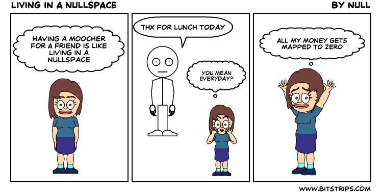
review 2.8 and
nullspace
Clicker questions in 2.8
Catalog description: A study of vectors, matrices and linear
transformations, principally in two and three dimensions,
including
treatments of systems of linear equations, determinants,
and
eigenvalues.
-Eigenvalues and applications (2.8, 5.1 and 5.6) (after test 3: chap 7
selections)
Begin 5.1:
the algebra of eigenvectors and eigenvalues, and connect to geometry and
Maple.
Begin 5.6: Eigenvector
decomposition for a diagonalizable matrix A_nxn
[where the eigenvectors form a basis for all of Rn]
Application: Foxes and Rabbits
Tues June 15 Test 2. Resume class at 3:50.
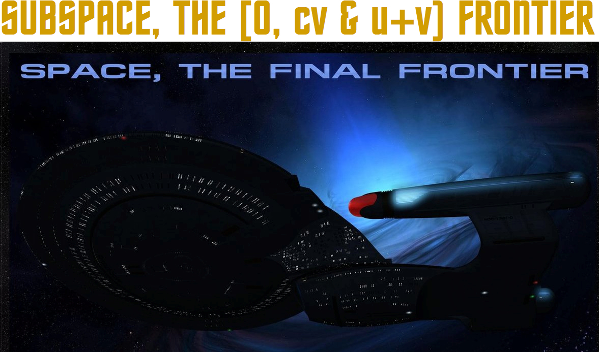
subspace,
basis, null space and column space
2.8 using the matrix 123,456,789 and finding the Nullspace and
ColumnSpace (using 2 methods - reducing the spanning equation with a vector
of b1...bn, and separately by examining the pivots of the ORIGINAL matrix.)
Two other examples.
Mon Jun 14
Clicker questions in Chapter 3 #3-8
3.3 p. 180-181:
The relationship of row operations to the
geometry of determinants - row operations can be seen as vertical
shear matrices
when written as elementary matrix form, which preserve area, volume, etc...
Overview of new material for test 2
Fri Jun 13
Clicker questions in Chapter 3 #1 and 2
Chapter 3 in Maple via MatrixInverse command for 2x2 and 3x3 matrices and
then determinant work, including 2x2 and 3x3 diagonals methods,
and Laplace's expansion (1772 - expanding on Vandermonde's
method) method in general. [general history dates to Chinese and Leibniz]
M:=Matrix([[a,b,c],[d,e,f],[g,h,i]]);
Determinant(M); MatrixInverse(M);
M:=Matrix([[a,b,c,d],[e,f,g,h],[i,j,k,l],[m,n,o,p]]);
Determinant(M); MatrixInverse(M);
LaTex Beamer slides
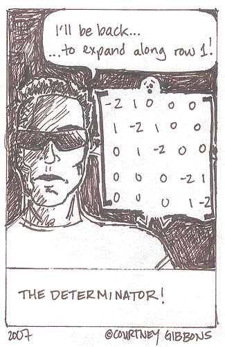
Review the 2 determinant methods for the 123,456,789 matrix. Show that
for 4x4 matrix in Maple, only Laplace's method will work.
The determinator comic
The connection of row operations to determinants
The determinant of A transpose and A triangular (such as in
Gaussian form).
The determinant of A inverse via the determinant of the product
of A and A inverse - and via elementary row operations -
so det A non-zero can be added into Theorem 8 in Chapter 2:
What Makes a Matrix Invertible.
Mention google searches:
application of determinants in physics
application of determinants in economics
application of determinants in chemistry
application of determinants in computer science
Eight queens and determinants
application of determinants in geology: volumetric strain
Thur Jun 12
Review linear transformations of
the plane, including homogeneous coordinates.
linear transformations comic
Finish linear transformation of the plane
Computer graphics demo [2.7]
Clicker questions in 2.7 #3 and 4
Keeping a car on a
racetrack
Clicker questions in 2.7 #5-7
Begin Yoda (via the file yoda2.mw) with data from Kecskemeti B. Zoltan
(Lucasfilm LTD) as on
Tim's page
Clicker questions in 2.7 #8
Linear transformations of 3-space:
Computer graphics demo [2.7]
Wed Jun 11
Review What Makes a Matrix Invertible
Clicker questions in 2.7 #1 and 2
Applications of 2.1-2.3:
1.8 (p. 62, 65, & 67-68), 1.9 (p. 70-75), and 2.7
Finish
Guess the transformation
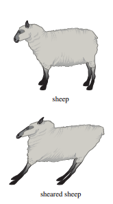
Mirror mirror and Sheared Sheap
general geometric transformations on
R2 [1.8, 1.9]
In the process, review the unit
circle
Computer graphics demo [2.7]
Tues Jun 10
Clicker questions in 2.3 and Hill Cipher # 1
(which is like 2.2 # 21 and 23)
Mention 2.1 #21 and 23 and
What Makes a Matrix Invertible
Clicker questions in 2.3 and Hill Cipher
# 2 and 3
Linear transformations: Ax=b where A is fixed but b varies:
1 unique solutions, 0 and infinite solutions, and 0 and 1 solutions.
Ax=0 with 1 or infinite solutions, depending on A.
Finish 2.3 via the condition number:
Maple file on Hill Cipher and
Condition Number and
PDF version
Computer graphics and linear transformations (1.8, 1.9, 2.3 and 2.7):
Guess the transformation
Mon Jun 9
Test 1 corrections
Clicker questions in 2.1 continued with
#7 and 8
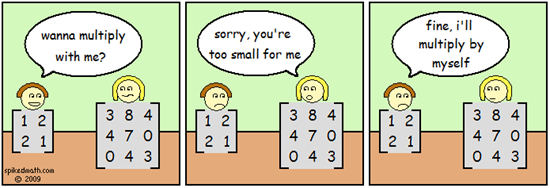
multiply comic, identity comic
Clicker questions in 2.2 #1 and 2
Theorem 8 in 2.3 [without linear transformations]: A matrix has a unique
inverse, if it exists. A matrix with an inverse has Ax=b with unique solution x=A^(-1)b, and then the columns span and are l.i...
What makes a matrix invertible
Discuss what it means for a square matrix that violates one of the
statements. Discuss what it means for a matrix that is not square (all bets
are off) via counterexamples.
-2.1-2.3 Applications: Hill Cipher, Condition Number and Linear
Transformations (2.3, 1.8, 1.9 and 2.7)
Applications: Introduction to Linear Maps
The black hole matrix: maps R^2 into the plane but not onto (the range
is the 0 vector).
Dilation by 2 matrix
Linear transformations in the cipher setting:
| A |
B |
C |
D |
E |
F |
G |
H |
I |
J |
K |
L |
M |
N |
O |
P |
Q |
R |
S |
T |
U |
V |
W |
X |
Y |
Z |
| 1 |
2 |
3 |
4 |
5 |
6 |
7 |
8 |
9 |
10 |
11 |
12 |
13 |
14 |
15 |
16 |
17 |
18 |
19 |
20 |
21 |
22 |
23 |
24 |
25 |
26 |
Applications of 2.1-2.3:
Hill Cipher history
Maple file on Hill Cipher and
Condition Number and
PDF version
Fri Jun 6
Multiplicative Inverse for 2x2 matrix:
twobytwo := Matrix([[a, b], [c, d]]);
MatrixInverse(twobytwo);
MatrixInverse(twobytwo).twobytwo
simplify(%)
2.2 Algebra: Inverse of a matrix.
Repeated methodology: multiply by the inverse on both sides, reorder by
associativity, cancel A by its inverse, then reduce by the identity to
simplify:
Applications of multiplication and the inverse
(if it exists).
Thur Jun 5
matrix multiplication and
matrix algebra. AB not BA...
Introduce
transpose of a matrix via Wikipedia, including Arthur Cayley.
Applications including least squares estimates, such as in linear regression,
data given as rows (like Yoda).
Test 1 review
Take review questions for test 1
Wed Jun 4
s13n15extension:=Matrix([[1,-5,b1],[3,-8,b2],[-1,2,b3]]);
GaussianElimination(s13n15extension);
Clicker questions in 1.3 # 4 and 5
discuss what happens when we correctly use
GaussianElimination(s13n15extension) - write out the equation of the plane
that the vectors span. Choose a vector that violates this equation to
span all of R^3 instead of the plane and plot:
M:=Matrix([[1,-5,0,b1],[3,-8,0,b2],[-1,2,1,b3]]);
GaussianElimination(M);
a:=spacecurve({[t, 3*t, -1*t, t = 0 .. 1]}, color = red, thickness = 2):
b:=spacecurve({[-5*t, -8*t, 2*t, t = 0 .. 1]}, color = blue, thickness
= 2):
diagonalparallelogram:=spacecurve({[-4*t, -5*t, -1*t, t = 0 .. 1]},
color = black, thickness = 2):
c:=spacecurve({[0, 0, t, t = 0 .. 1]}, color = magenta, thickness = 2):
display(a,b,c,d);
Clicker questions in 1.7 (and l.i.
equivalences)
In R^2: spans R^2 but not li, li but does not span R^2
Begin Chapter 2:
Continue via Clicker questions in 2.1 1-6
Image 1
Image 2
Image 3
Image 4
Image 5
Image 6
Image 7.
Matrix multiplication
Tues Jun 3
Linearly independent and span checks:
li1:= Matrix([[1, 4, 7,0], [2, 5,8,0], [3, 6,9,0]]);
ReducedRowEchelonForm(li1);
span1:=Matrix([[1, 4, 7, b1], [2, 5, 8,b2], [3, 6, 9,b3]]);
GaussianElimination(span1);
Plotting - to check whether they are in the same plane:
a1:=spacecurve({[t, 2*t, 3*t, t = 0 .. 1]}, color =
red, thickness = 2):
a2:=textplot3d([1, 2, 3, ` vector [1,2,3]`], color = black):
b1:=spacecurve({[4*t,5*t,6*t,t = 0 .. 1]}, color = green, thickness = 2):
b2:=textplot3d([4, 5, 6, ` vector [4,5,6]`], color = black):
c1:=spacecurve({[7*t, 8*t, 9*t, t = 0 .. 1]},color=magenta,thickness = 2):
c2:=textplot3d([7,8,9,`vector[7,8,9]`],color = black):
d1:=spacecurve({[0*t,0*t,0*t,t = 0 .. 1]},color=yellow,thickness = 2):
d2:=textplot3d([0,0,0,` vector [0,0,0]`], color = black):
display(a1, a2, b1, b2, c1, c2, d1, d2);
Linear Combination check of
adding a vector that is outside the plane containing Vector([1,2,3]), Vector([4,5,6]), Vector([7,8,9]), ie b3+b1-2*b2 not equal to 0: Vector([5,7,10] as opposed to [5,7,9])
M:=Matrix([[1, 4, 7, 5], [2, 5, 8, 7], [3, 6, 9, 10]]);
ReducedRowEchelonForm(M);
Span check with additional vector:
span2:=Matrix([[1, 4, 7, 5,b1], [2, 5, 8,7,b2], [3, 6, 9,10,b3]]);
GaussianElimination(span2);
Linearly independent check with additional vector:
li2:= Matrix([[1, 4, 7, 5,0], [2, 5, 8,7,0], [3, 6, 9,10,0]]); ReducedRowEchelonForm(li2);
Removing Redundancy
li3:= Matrix([[1, 4, 5,0], [2, 5,7,0], [3, 6,10,0]]); ReducedRowEchelonForm(li3);
Adding the additional vector to the plot:
e1:=spacecurve({[5*t,7*t,10*t,t = 0 .. 1]},color=black,thickness = 2):
e2:=textplot3d([5,7,10,` vector [5,7,10]`], color = black):
display(a1, a2, b1, b2, c1, c2, d1, d2,e1,e2);
Mon Jun 2
Clicker questions in 1.3 # 1, 2
and 3.
Clicker question in 1.4
Coff:=Matrix([[.3,.4,36],[.2,.3,26],[.2,.2,20],[.3,.1,18]]);
ReducedRowEchelonForm(Coff);
Coffraction:=Matrix([[3/10,4/10,36],[2/10,3/10,26],[2/10,2/10,20],[3/10,1/10,18]]);
ReducedRowEchelonForm(Coffraction);
Decimals (don't use in Maple) and fractions. Geometry of the columns as a plane in R^4, of the rows as 4
lines in R^2 intersecting in the point (40,60).
1.5: vector parametrization equations of homogeneous and non-homogeneous
equations. Introduce t*vector1 + vector2 is the collection of vectors
that end on the line parallel to vector 1 and through the tip of vector 2
1.7 definition of linearly independent and
connection to efficiency of span:
Clicker questions in 1.7 (and l.i.
equivalences)
In R^2: spans R^2 but not li, li but does not span R^2, li plus spans R^2.
Fri May 30 Collect problem set 1. Register remaining iclickers.
Review the language of vectors, scalar mult and addition, linear combinations and weights, vector equations and connection to 1.1 and 1.2 systems of equations and augmented matrix, and span.
Review that c1*vector1 + c2*vector2_on_a_different_line is a plane via:
span1:=Matrix([[1, 4, b1], [2, 5, b2], [3, 6, b3]]);
GaussianElimination(span1);
a1:=spacecurve({[t, 2*t, 3*t, t = 0 .. 1]}, color = red, thickness = 2):
a2:=textplot3d([1, 2, 3, ` vector [1,2,3]`], color = black):
b1:=spacecurve({[4*t,5*t,6*t,t = 0 .. 1]}, color = green, thickness = 2):
b2:=textplot3d([4, 5, 6, ` vector [4,5,6]`], color = black):
c1:=spacecurve({[7*t, 8*t, 9*t, t = 0 .. 1]},color=magenta,thickness = 2):
c2:=textplot3d([7,8,9,`vector[7,8,9]`],color = black):
Begin 1.4. Ax via using weights from x for columns of A versus Ax via dot
products of rows of A with x and Ax=b the same (using definition 1 of linear
combinations of the columns) as the augmented matrix [A |b]. The matrix
vector equation and the augmented matrix.
The matrix vector equation and the augmented matrix
and the connection of mixing to span and linear
combinations.
Theorem 4 in 1.4
Thur May 29 Collect hw and take questions.
Clicker questions 1.1 and 1.2 continued
with #2 onward:
Parametrize x+y+z=1.
History of linear equations and the term "linear algebra"
images, including the Babylonians 2x2 linear
equations, the
Chinese 3x3 column elimination method over 2000 years ago, Gauss' general
method arising from geodesy and least squares methods for celestial
computations, and Wilhelm Jordan's contributions.
Gauss quotation. Gauss was also involved in
other linear algebra, including the
history of vectors, another important "linear" object.
vectors, scalar mult and addition,
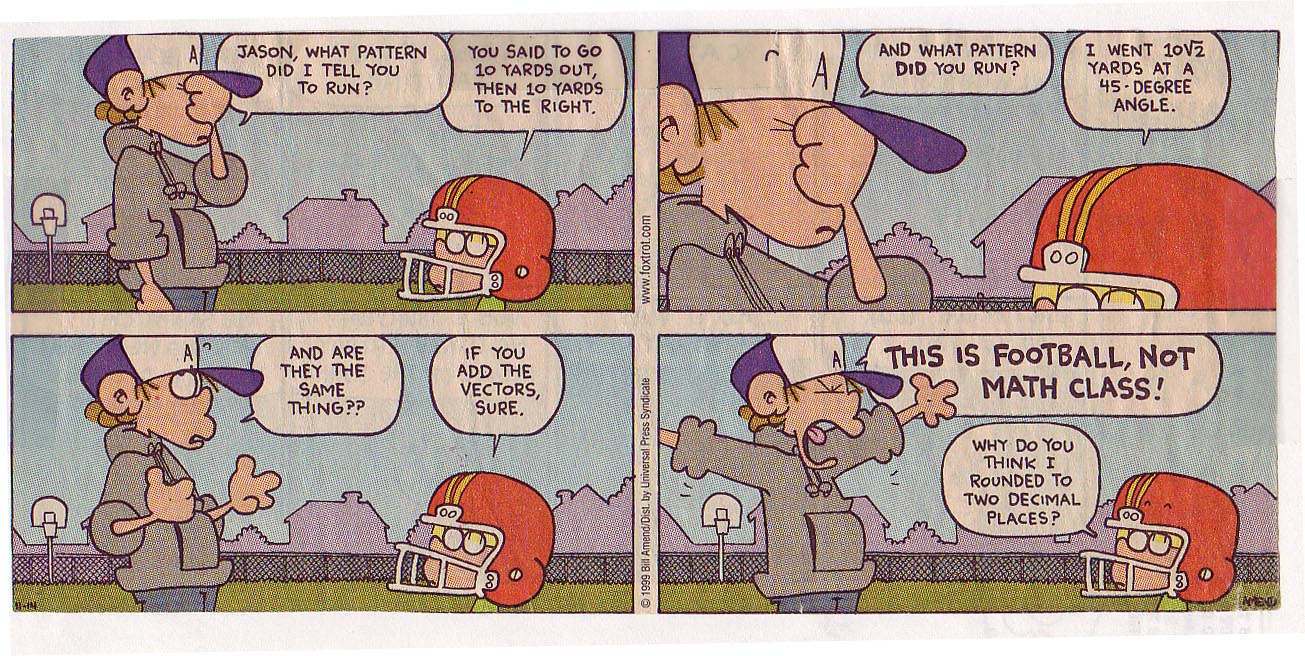
Foxtrot vector addition comic by
Bill Amend. November 14, 1999. linear combinations and weights,
vector equations and connection to 1.1 and 1.2 systems of equations and
augmented matrix. linear combination language (addition and scalar
multiplication of vectors).
Wed May 28
Turn in hw.
Register the i-clickers.
Clicker questions 1.1 and 1.2 #1.
Mention solutions and a glossary on ASULearn.
Prepare to share your name, major(s)/minors/concentrations, and
something you learned from hw or class yesterday or had a question on.
Review Gaussian and Gauss-Jordan for 3
equations and 2 unknowns in R2.
Gaussian and Gauss-Jordan or reduced
row echelon form in general:
section 1.2, focusing on algebraic and geometric perspectives
and solving using by-hand elimination of systems of equations with 3
unknowns. Follow up with
Maple commands and visualization: ReducedRowEchelon and
GaussianElimination as well as implicitplot3d in Maple (like on the
handout):
with(plots): with(LinearAlgebra):
Ex1:=Matrix([[1,-2,1,2],[1,1,-2,3],[-2,1,1,1]]);
implicitplot3d({x-2*y+z=2, x+y-2*z=3, (-2)*x+y+z=1}, x = -4 .. 4, y = -4 .. 4, z = -4 .. 4)
Ex2:=Matrix([[1,2,3,3],[2,-1,-4,1],[1,1,-1,0]]);
implicitplot3d({x+2*y+3*z=3,2*x-y-4*z=1,x+y-z=0},
x=-4..4,y=-4..4,z=-4..4);
Ex3:=Matrix([[1,2,3,0],[1,2,4,4],[2,4,7,4]]);
implicitplot3d({x+2*y+3*z = 0, x+2*y+4*z = 4, 2*x+4*y+7*z = 4}, x = -13 .. -5, y = -1/4 .. 1/4, z = 3 .. 5, color = yellow)
Ex4:=Matrix([[1,3,4,k],[2,8,9,0],[10,10,10,5],[5,5,5,5]]); GaussianElimination(Ex4);
Highlight equations with 3 unknowns with infinite solutions, one solution
and no
solutions in R3, and the corresponding geometry, as we review
new terminology and glossary words.
Tues May 27
UTAustinXLinearAlgebra.mov
History of solving equations
1.1 Work on the introduction to linear algebra handout motivated from
Evelyn Boyd Granville's favorite
problem (#1-3).
At the same time, begin 1.1 (and some of the words in 1.2)
including geometric perspectives,
by-hand algebraic Gaussian
Elimination and pivots,
solutions, plotting and geometry, parametrization and GaussianElimination
in Maple for systems with 2 unknowns in R2.
Evelyn Boyd Granville #3:
with(LinearAlgebra): with(plots):
implicitplot({x+y=17, 4*x+2*y=48},x=-10..10, y = 0..40);
implicitplot({x+y-17, 4*x+2*y-48},x=-10..10, y = 0..40);
EBG3:=Matrix([[1,1,17],[4,2,48]]);
GaussianElimination(EBG3);
ReducedRowEchelonForm(EBG3);
Course intro slides
Do EBG#4
Evelyn Boyd Granville #4
EBG4:=Matrix([[1,1,a],[4,2,b]]);
GaussianElimination(EBG4);
3 equations and 2 unknowns in
R2
Gaussian and EBG#5
with
k as an unknown but constant coefficient:
EBG5:=Matrix([[1,k,0],[k,1,0]]);
GaussianElimination(EBG5);
ReducedRowEchelonForm(EBG5);
Prove using geometry of lines
that the number of solutions of a system
with 2 equations and 2 unknowns is 0, 1 or infinite.
Solve the system x+y+z=1 and x+y+z=2 (0 solutions - 2 parallel planes)
implicitplot3d({x+y+z=1, x+y+z=2}, x = -4 .. 4, y = -4 .. 4, z = -
4 .. 4)
How to get to the main calendar page: google Dr. Sarah /
click on webpage / then 2240
Review the following vocabulary,
which is also on the ASULearn glossary that I am experimenting with.
augmented matrix
coefficients
consistent
free
Gaussian elimination / row echelon form (in Maple GaussianElimination(M))
Gauss-Jordan elimination / reduced row echelon form (in Maple ReducedRowEchelonForm(M))
homogeneous system
implicitplot
implicitplot3d
linear system
line
parametrization
pivots
plane
row operations / elementary row operations
solutions
system of linear equations
unique